
|
IFS( ): The IFS function checks whether one or more conditions are met and returns a value that corresponds to the first TRUE condition. IFS can take the place of multiple nested IF statements and is much easier to read with multiple conditions. Syntax: IFS([Something is True1, Value if True1, [Something is True2, Value if True2],…[Something is True127, Value if True127]) Notes: In MS-Excel, when you try to make conditions for logical testing, the IFS function allows you to test up to 127 different conditions. For example: Which says IF(A1 equals 0, then display 10, IF A1 equals 10, then display 100, or else if A1 equals 20, then display 200. It's generally not advisable to use too many conditions with IF or IFS statements, as multiple conditions need to be entered in the correct order, and can be very difficult to build, test and update. Remarks:
OK let me give conditions to find the result: As shown in the screenshot down, In Average column: E3>100 Then Wrong : E3>=85 Then A : E3>=60 Then B : E3>=50 Then C : E3>=35 Then S : E3<35 Then Fail Q: How to find the result in order to above conditions for the student’s average of the marks? Type the function as follows in the cell that you would like to get the result in: =IFS(E3>100, "WRONG", E3>=85,"A", E3>=60,"B", E3>=50,"C", E3>=35,"S", E3<35,"FAIL") For more understanding, look at the screenshot please: 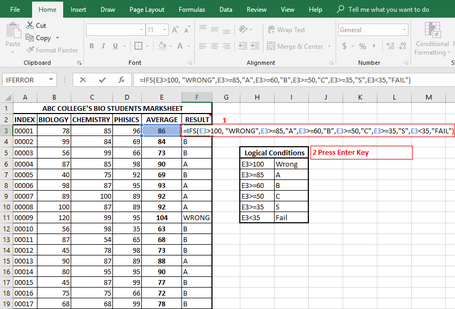 SWITCH( ): I have given about the formula syntax and usage of SWITCH, one of the logical functions in MS-Excel 2016. Note: This feature is only available if you have an MS-Office 365 subscription. If you are an MS-Office 365 subscriber, make sure you have installed latest version of MS-Office. The SWITCH function evaluates one value (called the expression) against a list of values, and returns the result corresponding to the first matching value. If there is no match, an optional default value may be returned. Syntax: SWITCH(Value to switch, Value to match1...[2-126], Value to return if there's a match1...[2-126], Value to return if there's no match) When you try to evaluate the matching, you can go up to 126 matching values and results. OK lets me give an example question and answer for the easy of understanding: Q: How to find the matched word whether is “MyDell” or “MyCap” or “MyCopy” in the Cell A3, If there is one of the matched word then result should be “Yes” or “No”? Type the function as follows in the cell that you would like to get the result in: =SWITCH(A3,"MyDell","Yes","MyCopy","Yes","MyCap","Yes","No") For more understanding, look at the screenshot please: 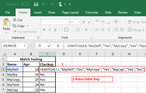
0 Comments
|
Archives |
 RSS Feed