
|
Insert Functions (Shift+F3): Note: You can work with the formula in the current cell and can easily pick functions to use and get expected outcome from function as well. SUM( ): Note: This function is being used to find the total of number from selected range of cells they are included only numbers. How to use Sum function to find the total of attendance students to selected three cells? Keep the cursor in a cell that you want to get the result => Select Formula Menu => Click Insert Function Tool => Select Sum in the section for functions => Click OK => Type your range of values cell addresses (C2:C4) => Click OK. For more understanding, look at the screenshot please: 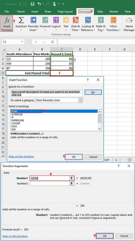 SUMIF( ) Function: You use the SUMIF function to sum the values in a range that meet criteria that you specify. For example, suppose that in a column that contains numbers, you want to sum only the values that are larger than 79. Syntax: SUMIF(range, criteria, [sum_range]) The SUMIF function syntax has the following arguments: Range Required. The range of cells that you want evaluated by criteria. Cells in each range must be numbers or names, arrays, or references that contain numbers. Blank and text values are ignored. Criteria Required. The criteria in the form of a number, expression, a cell reference, text, or a function that defines which cells will be added. For example, criteria can be expressed as 32, ">32", B5, "32", "apples". Important: Any text criteria or any criteria that includes logical or mathematical symbols must be enclosed in double quotation marks ("). If the criteria is numeric then only double quotation marks are not required. Sum_range Optional. The actual cells to add, if you want to add cells other than those specified in the range argument. If the sum_range argument is omitted, Excel adds the cells that are specified in the range argument (the same cells to which the criteria is applied). Remarks The SUMIF function returns incorrect results when you use it to match strings longer than 255 characters or to the string #VALUE!. Q: How to calculate the pass marks only with passed over “79” in all four subjects in the marks sheet? Type the function as follows in the cell that you would like to get the result in: =SUMIF(B3:E3,”>=80”, B3:E3) For more understanding, look at the screenshot please: 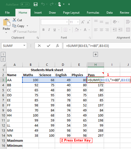 SUMIFS( ) function: The SUMIFS function, one of the math and trig functions, adds all of its arguments that meet multiple criteria. For example, you would use SUMIFS to sum the number of retailers in the country who (1) reside in a single zip code and (2) whose profits exceed a specific Rs value. Syntax SUMIFS(sum_range, criteria_range1, criteria1, [criteria_range2, criteria2], ...) Sum_range (required) The range of cells to sum. Criteria_range1 (required) The range that is tested using Criteria1. Criteria_range1 and Criteria1 set up a search pair whereby a range is searched for specific criteria. Once items in the range are found, their corresponding values in Sum_range are added. Criteria1 (required) The criteria that defines which cells in Criteria_range1 will be added. For example, criteria can be entered as 50, ">50", C4, "apples", or "50". Criteria_range2, criteria2, … (optional) Additional ranges and their associated criteria. You can enter up to 127 range/criteria pairs. Q: How to calculate the number of product that aren’t bananas and are sold by Vengad in the sales sheet? = Type the function as follows in the cell that you would like to get the result in: =SUMIFS(C2:C9, B2:B9, "<>Bananas", A2:A9, "Vengad") For more understanding, look at the screenshot please: 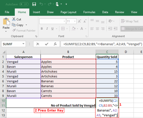
0 Comments
|
Archives |
 RSS Feed