
|
Average: Note: Returns the average (arithmetic mean) of the arguments. For example, if the range B3:B14 contains numbers, the formula =AVERAGE(B3:B14) returns the average of those numbers. Syntax AVERAGE(number1, [number2], ...) The AVERAGE function syntax has the following arguments: Number1 Required. The first number, cell reference, or range for which you want the average. Number2, ... Optional. Additional numbers, cell references or ranges for which you want the average, up to a maximum of 255. Remarks: Arguments can either be numbers or names, ranges, or cell references that contain numbers. Question: How to find the average of the Student Marks in Students Mark Sheet Table? Type the function as follows in the cell that you would like to get the result in: =average(B3:D3) For more understanding, look at the screenshot please: 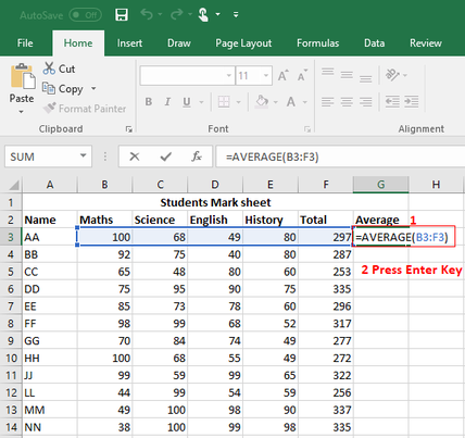 AVERAGEA function: I have given here about formula syntax and usage of the AVERAGEA function in Microsoft Excel. Description: Calculates the average (arithmetic mean) of the values in the list of arguments. Syntax: AVERAGEA(value1, [value2], ...) The AVERAGEA function syntax has the following arguments: Value1, value2, ... Value1 is required, subsequent values are optional. 1 to 255 cells, ranges of cells, or values for which you want the average. Logical values and text representations of numbers that you type directly into the list of arguments are counted. Arguments that contain TRUE evaluate as 1; arguments that contain FALSE evaluate as 0 (zero). Array or reference arguments that contain text evaluate as 0 (zero). Empty text ("") evaluates as 0 (zero). Remarks: Arguments can be the following: numbers; names, arrays, or references that contain numbers; text representations of numbers; or logical values, such as TRUE and FALSE, in a reference. Note: The AVERAGEA function measures central tendency, which is the location of the center of a group of numbers in a statistical distribution. The three most common measures of central tendency are: Average: which is the arithmetic mean and is calculated by adding a group of numbers and then dividing by the count of those numbers. For example, the average of 14, 6, 13, 8, 9, and 10 is 60 divided by 6, which is 10. Median: which is the middle number of a group of numbers; that is, half the numbers have values that are greater than the median, and half the numbers have values that are less than the median. For example, the median of 2, 3, 3, 5, 7, and 10 is 4. Mode: which is the most frequently occurring number in a group of numbers. For example, the mode of 2, 3, 3, 5, 7, and 10 is 3. Q: How to find the central tendency, which is the location of the center of a group of numbers that those are already entered in worksheet? Type the function as follows in the cell that you would like to get the result in: =AVERAGEA(C2:C4) For more understanding, look at the screenshot please: 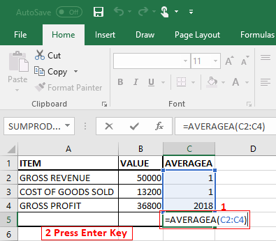 AVERAGEIF function: I have given about formula syntax and usage of the AVERAGEIF function in Microsoft Excel. Description: Returns the average (arithmetic mean) of all the cells in a range that meet a given criteria. Syntax: AVERAGEIF(range, criteria, [average_range]) The AVERAGEIF function syntax has the following arguments: Range: Required. One or more cells to average, including numbers or names, arrays, or references that contain numbers. Criteria: Required. The criteria in the form of a number, expression, cell reference, or text that defines which cells are averaged. For example, criteria can be expressed as 32, "32", ">32", "apples", or B4. Average_range Optional. The actual set of cells to average. If omitted, range is used. Remarks: Cells in range that contain TRUE or FALSE are ignored. If a cell in average_range is an empty cell, AVERAGEIF ignores it. If range is a blank or text value, AVERAGEIF returns the #DIV0! error value. Q: How to calculate the number of product that aren’t bananas and are sold by Vengad in the sale sheet? Type the function as follows in the cell that you would like to get the result in: =AVERAGEIF(B3:E3,">=80",B3:E3) For more understanding, look at the screenshot please: 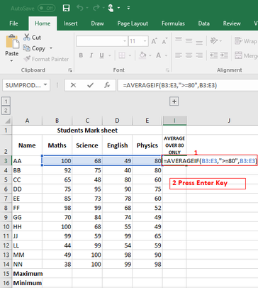 AVEDEV function: I have given here about formula syntax and usage of the AVEDEV function in Microsoft Excel. Description: Returns the average of the absolute deviations of data points from their mean. AVEDEV is a measure of the variability in a data set. Syntax: AVEDEV(number1, [number2], ...) The AVEDEV function syntax has the following arguments: Number1, number2, ... Number1 is required, subsequent numbers are optional. 1 to 255 arguments for which you want the average of the absolute deviations. You can also use a single array or a reference to an array instead of arguments separated by commas. Remarks: AVEDEV is influenced by the unit of measurement in the input data. Arguments must either be numbers or be names, arrays, or references that contain numbers. Logical values and text representations of numbers that you type directly into the list of arguments are counted. If an array or reference argument contains text, logical values, or empty cells, those values are ignored; however, cells with the value zero are included. Q: How to find average of the absolute deviation of data point for given value? Type the function as follows in the cell that you would like to get the result in: =AVEDEV(50,10) For more understanding, look at the screenshot please: 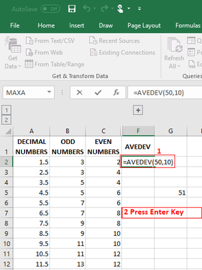
0 Comments
|
Archives |
 RSS Feed