
|
Numbers: Apparently in MS-Excel, you can use number formats to change the appearance of numbers, including dates and times, without changing the actual number. The number format does not affect the cell value that Excel uses to perform calculations. The actual value is displayed in the formula bar. MS-Excel provides several built-in number formats. You can use these built-in formats as is, or you can use them as a basis for creating your own custom number formats. When you create custom number formats, you can specify up to four sections of format code. These sections of code define the formats for positive numbers, negative numbers, zero values, and text, in that order. The sections of code must be separated by semicolons (;). How to change certain format of cells to currency sign “Rs”? Select cells that you want to change the format => Select Home Menu => Click General dropdown button => Click More Number Formats => Select Currency in the category section => Select Rs, Tamil (Sri Lankan) in the symbol dropdown button => Click OK. For more understanding, look at the screenshot please: 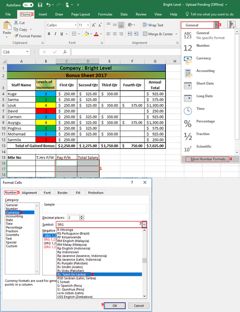 Conditional Formatting: For example, you have a worksheet with thousands of rows of data. It would be extremely difficult to see patterns and trends just from examining the raw information. Similar to charts and sparklines, conditional formatting provides another way to visualize data and make worksheets easier to understand. The Conditional formatting quickly highlights important information in a spreadsheet. But sometimes the built-in formatting rules don’t go quite far enough to fulfill our conditional goals. So, adding your own formula to a conditional formatting rule gives it a power boost to help you do things the built-in rules can’t do. Let’s say, you may choose to enter values into a conditional formatting to the cells, you can create rules of conditional related to your data that you have. When you enter the data for between numbers, for example students marks and it should be min 1 to max 100 in each subject. so, how to create a conditional with formatting visual different for between numbers min1- max 100 to enter the data into cells? Select Cells that you want to create conditional => Select Home Menu => Click Conditional Formatting Tool => Select Highlight Cells Rules => Click Between => Type 1 in the first blank box and type 100 in second blank box and then Select a format colour “Ex: Light Red Fill” => Click OK. For more understanding, look at the screenshot please: 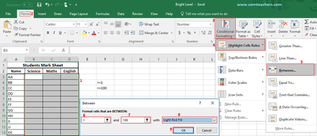
0 Comments
|
Archives |
 RSS Feed